Find the orthodox that contains a point

This article shows how to classify a set of high -dimensions data into orthodox. An orthlant is the d-dimensional generalization of a quadrant.

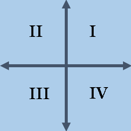
For the 2-D Euclidian space, there are four quadrants, often labeled by Roman I-IV numbers. Quadrants are open groups that are determined by the signs of each coordinate of a point (x1, x2). Traditionally, quadrants are recorded to the right from the positive X axis, as follows:

• I: The first quadrant is determined by {(x1, x2) | x1> 0 and x2> 0. Coordinate signs are ‘++’.
• II: The second quadrant is determined by {(x1, x2) | x1 <0 dhe x2> 0. Coordinate signs are ‘-+’.
• III: The third quadrant is determined by {(x1, x2) | x1 <0 and x2 <0. The signs of the coordinates are '-'.
• IV: Fourth quadrant is determined by {(x1, x2) | x1> 0 and x2 <0. Coordinate signs are '+-'.

In higher dimensions, there is no convention on how to count the orthodox, which are generalized quadrants. So let’s create our own tag scheme that uses the signs of coordinates to give each orthodox a unique label. You can accompany a positive sign (‘+’) with 1 and a negative sign (‘-‘) with 0. You can turn binary representation into a full number 0 to 2^mud–1 in a natural way.

For example, 2-D quadrants are associated with figures 0-3 through strings ’00’, ’01’, ’10’ and ’11’. Since we usually count starting from 1, it is common to add 1 to each octant to obtain numbers 1-4. Note that this produces a different tag group rather than learned in high school:

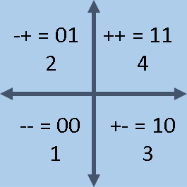
• ‘++’ string is designed to ’11’. On the binary, this range is equal to 3. Add 1 to that value. Thus, the quadrant with ‘++’ signs is called Quadrant 4 with this new method of labeling.
• The ‘-+’ string is compiled on ’01’. On the binary, this range is equal to 1. Add 1 to that value. Thus, the quad with the ‘-+’ signs is called quadrant 2 with this method of labeling.
• Similarly, the quadrant with ‘-‘ is called Quadrant 1, and quadrant with ‘+-‘ signs is called quadrant 3.

In a similar way, an orth time in the 3-D space is called a octant. You can classify a 3-D point into an octant by looking at the signs of the three coordinates of a point. Octants are determined by the following eight signs trio: ‘+++’, ‘++-‘, ‘+-+’, ‘+-‘, ‘-++’, ‘-+-‘, ‘-+’, and ‘—‘. Binary values ​​are 7 to 0 (in descending order), so the labels are 8 to 1.

In general, orthodox in the Euclidian D-dimensional space are determined by the set of unique wires in two symbols. Group size is 2^mudand has a one-to-one natural correspondence with integers 0 to 2^mud–1 when written at base-2 (binary). Thus, we can label the orthodox with integers 1 to 2^mud.

Why do we care what orthodox point is a point?

This current article is motivated by an latest project in which I reviewed a simulation algorithm that is supposed to create high -dimensional dimensions that are spherically symmetrical. In an accurate simulation, each point of synthetic data has an equal probability to appear in any orthodox. Showing the distribution of the orthodox, I was able to tell the author that his algorithm was incorrect.

To understand the relationships between spherical symmetry and the orthodox, let’s think briefly about the 2-D data. Suppose you are given a set of two-dimensional observations. By subtracting the average (or average) of each variable, you can concentrate the data related to the origin. Now, assume that you label you any observation for data concentrated according to its Euclidian quad. This tells you some things about data distribution:

• If the observations approximately N/4 are in each quadrant, then the data is unrelated or poorly related.
• If most observations are in quadrants I and III, the data is positively connected.
• If most observations are in quadrants II and IV, the data is negatively connected.

Thus, the distribution of orthodox for concentrated data is a way to examine whether the data distribution is spherically symmetrical or whether there are correlations in the data.

A first look at the point classification in orthodox

Suppose you have a series of 2-D points. How can you identify the quad for each point? One way is to use the sign function in SAS, which returns the value -1 if a value is negative, +1 if the value is positive, and 0 if the value is 0. The sign function in the data step gets a scalar argument, but remember that you can call the SAS functions from ProMl and switch to vectors or matrix.

The following IML program defines a matrix, where each line is a point at 2-D. In this example, there is one point in each quadrant. To find the quadrant, you can use the sign function to design the coordinates in a 0/1 binary matrix. It is now the binary layout of a 0-3 number. You can turn the line into a base-10 number and add 1 to get the quadrant number. Mathematically the quadrant number for the row i_th is


\ (q_i = 1 + \ sum \ nollation_ {j = 0}^p b_ {ij} 2^i \)

where \ (b_ {ij} \) are binary values ​​0/1 in the line i_th. The program shows the quad for each point:

proc iml;
z = {
 7  8,    /* I   */
-6  8,    /* II  */
-2 -3,    /* III */
 5 -6 };  /* IV  */
 
d = ncol(z);
s = (sign(z) + 1) / 2;      /* sign(z) contains {-1,1}; map these values to {0,1} */
pow = 2##(d-1:0);           /* powers of 2 for d <= 53     */
quadrant = 1 + (s#pow)(,+); /* quadrant number for d <= 53 */
print z(c={'x1' 'x2'} r={I,II,III,IV} L='Convention') quadrant(L='New Label');

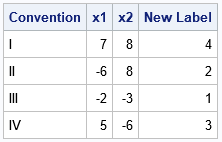
Production accurately classifies each point 2-D as in the first, second, third or fourth quadrant.

A function that classifies the points in orthodox

You can include these statements in a SAS IML function that calculates orthodox for points in each dimension (well, dimension cannot exceed 53 because 2^mud It should be represented as a full number, but this method is most useful for the smallest values ​​of d.) For the whole, the following function also deals with the case where a point coordinate is zero. In that case, the issue is not in any quadrant, so the function returns a lost value.

/* z is an (n x d) matrix of points, where d <= 53.
   Find the orthant that contains the point.
   Ex: z = {-1 1};
       q = CoordToOrthant(z);
   Answer is 3 because z is in the 3rd octant.
*/
start CoordToOrthant(z);
   s = sign(z);
   d = ncol(z);
   b = (s + 1) / 2;            /* sign(z) contains {-1,1}; map these values to binary {0,1} */
   w = 2##(d-1:0);             /* powers of 2 */
   orthant = 1 + (b#w)(,+);    /* convert binary representation to quadrant number */
   /* handle the zero-probability case where sign(z)=0 */
   idx = loc(s = 0);           /* are any points are on a subspace where x(i)=0 for some i? */
   if IsEmpty(idx) then    
      return orthant;          /* usual case; return quadrants */
   rc = ndx2sub(dimension(z), idx);   /* get rows and columns for the indices */
   orthant(rc(,1), ) = .;      /* set quadrant for those rows to missing */
   return orthant;
finish;
 
z = { 
 5  6  4,
 7  8 -9,
 3 -2  7,
 5 -6 -4,
-2  8  9,
-3  6 -4,
-6 -5  8,
-2 -3 -5,
 6  0  3 };   /* x2=0 */
 
octant = CoordToOrthant(z);
print z(c={'x1' 'x2' 'x3'}) octant;

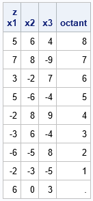
Production indicates that 3-D points are correctly classified into the octant, including the point in the last row, which is not in any octant.

Application: Distribution of Points in Orthodox

As mentioned earlier, this article is motivated by a project in which I had to appreciate if a simulation algorithm was generating accurate production. I knew that the correct output is spherically symmetrical, meaning that there is an equal probability that the points appear in each orthodox. Instead of examining data distribution, it was easier to examine the distribution of orthodox for the data.

For example, assume you want to simulate normal randomly unrelated changes. Simulated data is spherically symmetrical, so if you simulate data points B in dimensions D, approximately B/2^mud From them should be in each orthodox. Let’s execute an experiment by generating 8,000 randomly unrelated 3-D variants and plotting a bar of orthodox bar:

call randseed(123);
d = 3;
N = 2##d * 1000;
/* generate N uncorrelated random normal variates in d dimensions */
mu = j(1, d, 0);
Sigma = I(d);
Z = randnormal(N, mu, Sigma);
 
orthant = CoordToOrthant(Z);
title "Distribution of Uncorrelated 3-D Points in Octants";
call bar(orthant) grid="y";

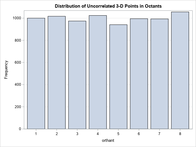
The ribbon graph shows that of the 8,000 random points, it has approximately 1,000 points in each of the eight octans in 3-D.

The graph of the drug looks different if the points are connected. At 2-D, a positively linked data distribution plot shows that most points are in the first and third quadrants. This geometry is generalized in higher dimensions. For example, the following statements of IML determine a 3 x 3 correlation matrix for which the variables (x1, x2) have a large positive correlation and the variables (x2, x3) have a large negative correlation.

/* contrast with the octants of strongly correlated data */
Sigma = { 1    0.7 -0.2,
          0.7  1   -0.7,
         -0.2 -0.7  1   };
 
X = randnormal(N, mu, Sigma);
orthant = CoordToOrthant(X);
title "Distribution of Correlated 3-D Points in Octants";
call bar(orthant) grid="y";

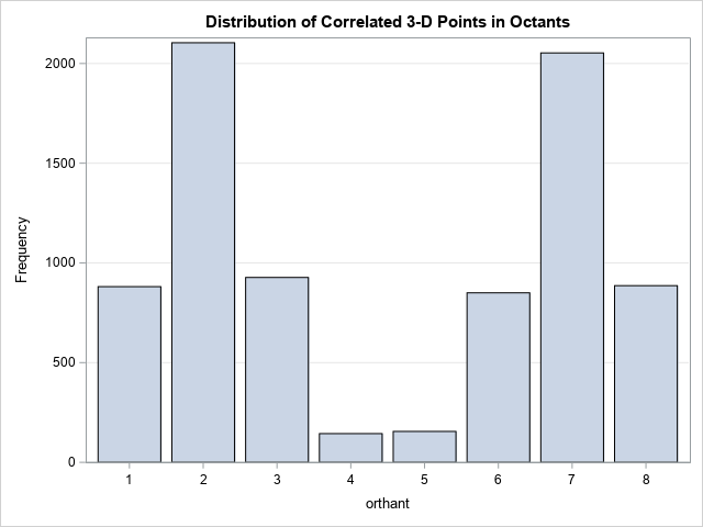
The ribbon graph indicates that the points do not distribute evenly to eight octants. There are many points in Octants 2 and 7, and relatively slightly in Octants 4 and 5.

Briefing

This article shows how to use the SAS sign function to calculate orthodox for a set of d-dimensional points. The function first uses the function of the sign to build a vector of coordinate sign. This vector is naturally designed in the basic representation of a number, which is designed in a integer in the 1-2 range^mud. This integer is the orthodox number. An application of this technique is to determine whether a sample with high dimensions of concentrated data is spherically symmetrical.