An application of Latin Hypercub Sampling for Optimization

A previous article discusses a “Catch-22” paradox for mounting nonlinear regression models: you cannot evaluate the parameters until you fit the model, but you cannot fit the model until you provide an initial assumption for the parameters! If your initial assumption of parameters is not good enough, the algorithm of nonlinear optimism that tries to maximize the logiclane may not converge. The previous article shows how to specify a network of initial parameters values ​​in Proc Nllin and Proc nlmixed. The procedures evaluate the model logic (ll) in each tuple parameters on the grid, then uses what has the largest logic as the initial assumption for optimization. Although we often talk about the maximum evaluation of the likelihood, many routines minimize negative logicelism. Thus, in this article, the best parameters are those that have smaller values ​​for the negative.

For example, assume you have five parameters in the model. If you specify 10 possible values ​​for each parameter, then the network of all parameters is the Cartesian product, which has 10⁵ = 100,000 tuple of parameters. The appropriate algorithm should evaluate ll at all these points before the process of optimism begins. If your data set is large and the model is complex, this can be an expensive calculation.

There is another option. The Proc Nlmixed Sauls statement supports a data option = that enables you to specify a set of data for which each line is a set of parameters values. (In ProC Nllin and SAS procedures, use the PDATA option =.) You can use Latin Hypercub Samples (LHS) in SAS to create a much smaller group that however explore the parameter space. In theory, you can achieve a similar value LL using much less tuples of the parameters. This article shows how to use LHS to select the initial assumptions for an optimization. This technique is often used in learning machinery and deep learning during a “hypertuning” step, which sets the parameters for an algorithm.

A nonlinear regression model

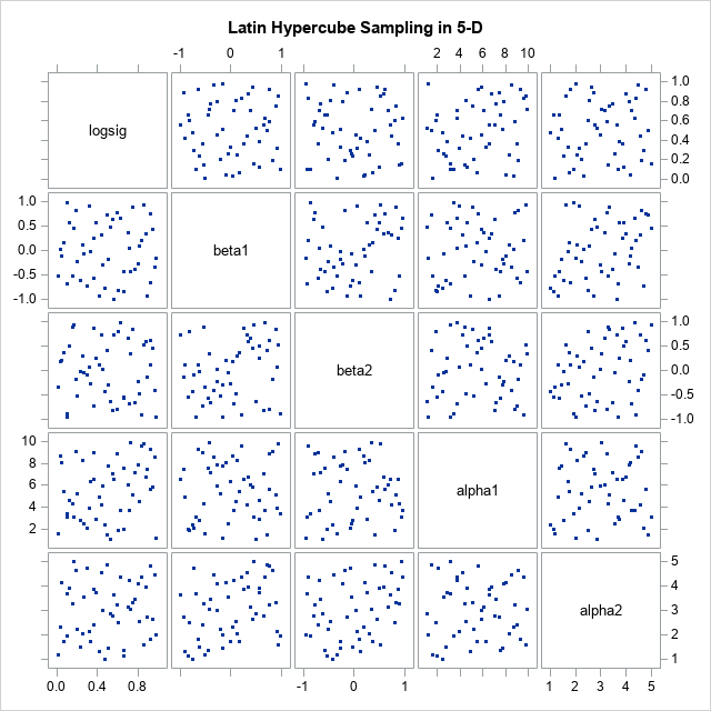
Let us use the same nonlinear regression problem from the previous article. The problem has five parameters. We want to select an initial set of parameters in the following range: Logsig in at (0, 1), beta1 and beta2 are in (-1, 1), alpha1 is in (1, 10), and Alfa2 is in (1, 5). The appendix defines and stores the SAS IML modules for performing the Latin hypercub samples. You can upload these modules and call them to create a LHS sample. Instead of hundreds or thousands of samples, let’s generate 50 initial assumptions, as follows:

proc iml;
/* load modules from Appendix. See also https://blogs.sas.com/content/iml/2024/12/09/latin-hypercube-sampling-sas.html */
load module=(UnifSampleSubIntervals PermuteRows LatinHyperSample); 
call randseed(1234);
/*           min  max     ParmName */
intervals = { 0    1,   /* logsig in (0,1)  */
             -1    1,   /* beta1 in (-1,1)  */
             -1    1,   /* beta2 in (-1,1)  */
              1   10,   /* alpha1 in (1,10) */
              1    5};  /* alpha2 in (1,5)  */
varNames = {'logsig' 'beta1' 'beta2' 'alpha1' 'alpha2'};
NumPts = 50;
LHS = LatinHyperSample(intervals, NumPts);
 
create ParamDataLHS from LHS(c=varNames);
append from LHS;
close;
quit;
 
title "Latin Hypercube Sampling in 5-D";
proc sgscatter data=ParamDataLHS;
   matrix logsig beta1 beta2 alpha1 alpha2 / markerattrs=(symbol=CircleFilled);
run;

The call for Proc Sgscatter provides a visualization of 50 five-dimensional points. Note that 2-D marginal distributions of points are approximately uniform.

The following data step determines the data for the model. The call to process nlmixed fits with a five -parameter model. The 50 points created by the LHS model are used to get an initial assumption for nonlinear optimization.

/* Data and NLMIXED code for nonlinear regression. See  
   https://blogs.sas.com/content/iml/2018/06/25/grid-search-for-parameters-sas.html
*/
data pump;
  input y t group;
  pump = _n_;
  logtstd = log(t) - 2.4564900;
  datalines;
 5  94.320 1
 1  15.720 2
 5  62.880 1
14 125.760 1
 3   5.240 2
19  31.440 1
 1   1.048 2
 1   1.048 2
 4   2.096 2
22  10.480 2
;
 
/* Use Latin hypercube sampling instead of dense grid for parameter search */
proc nlmixed data=pump;
   parms / DATA=ParamDataLHS;        /* read guesses for parameters from LHS data set */
   if (group = 1) then 
        eta = alpha1 + beta1*logtstd + e;
   else eta = alpha2 + beta2*logtstd + e;
   lambda = exp(eta);
   model y ~ poisson(lambda);
   random e ~ normal(0,exp(2*logsig)) subject=pump;
   ods select ParameterEstimates;
   ods output Parameters=_LL;
run; 
 
/* for visualization: add an ID variable */
data LL / view=LL;
   set _LL;
   ObsNum = _N_;
run;
/* Optional: examine min and mean of negative LL */
proc means data=LL;
   var NegLogLike;
run;
 
title "Loglikelihood for 50 Points from LHS";
proc sgplot data=LL;
   scatter x=ObsNum y=NegLogLike;
   yaxis values=(0 to 250 by 50) grid;
run;

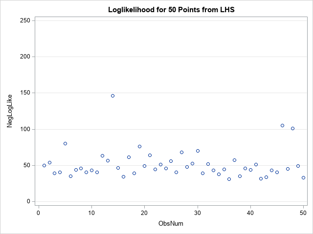
For the initial assumptions generated by the LHS, there are many whose negative values ​​are less than 50. The smallest negative value ll is 30.8. My previous article shows a similar graph for 300 points on a regular network. In that article, the smallest negative was 29.8, which means that the best initial assumption by the LHS method is comparable to the best assumption by the regular network method, while requires much less calculation. Of course, the LHS method has an element of chance, so there is no guarantee that the LHS method will provide a good starting assumption. However, the LHS method is often used in practice because it tends to perform well.

Why not use uniform random parameters?

Before learning about the sampling of Latin hypercub samples, I would often generate the random parameter uniformly in a 5-D hypercube. This is known as taking simple occasional samples, or SRS. The LHS method has some advantages to SRS. The main advantage is that LHS is guaranteed to explore all values ​​of each parameter. In contrast, SRS can result in gaps and clusters in several parameters. For casual coincidence, we can end with parameters that are all small or that contain no point in the middle of the range. In contrast, marginal empirical distributions of LHS points are guaranteed to be approximately uniform. By construction, if you use LHS to generate K samples, each of the sub-20s of equal length K for each coordinate will contain exactly one sample.

Briefing

This article shows how to use Latin Hypercube sampling (LHS) to generate initial conditions for an optimization that fits a nonlinear regression model in SAS. For this example, all parameters are continuous. However, the same technique can be used for hypertuning algorithms in machinery learning when some parameters must be discreet values. For discreet parameters, you can use the INT function to generate integer from the LHS method.

Appendix: SAS IML modules for taking Latin Hypercub Samples

For your convenience, the following SAS IML modules apply Latin hypercub samples. These modules are explained in the article “Sampling of Hypercube Latin in SAS”.

/* Latin Hypercube Sampling in SAS. See
   https://blogs.sas.com/content/iml/2024/12/09/latin-hypercube-sampling-sas.html
*/
proc iml;
/* UnifSampleSubIntervals:
   specify an interval (a,b) and a number of subintervals.
   Divide (a,b) into k subintervals and return a point uniformly at random 
   within each subinterval.
*/
start UnifSampleSubIntervals(interval, k);
   a = interval(1);
   b = interval(2);
   h = (b-a)/k;
   L = colvec( do(a, b-h/2, h) ); /* left-hand endpoints of k subintervals */
   u = randfun(k, "Uniform");     /* random proportion */
   eta = L + u*h;   /* eta(i) is randomly located in the i_th subinterval */
   return( eta );
finish;
 
/* PermuteRows helper function: Use the SAMPLE function to permute the rows of a matrix */
start PermuteRows(M);
   k = nrow(M);
   p = sample(1:k, k, "WOR");  /* random permutation of 1:k */
   return( M(p, ) );
finish;
 
/* LatinHyperSample:
   Generate random location in k subintervals for each of d intervals.
   intervals(i,) specifies the interval for the i_th coordinate
   k = (scalar) specifies the number of subintervals in each dimension 
*/
start LatinHyperSample(intervals, k); 
   d = nrow(intervals);
   LHS = j(k, d, .);
   do i = 1 to  d;
      eta = UnifSampleSubIntervals(intervals(i,), k);
      LHS(, i) = PermuteRows(eta);
   end;  
   return( LHS );
finish; 
store module=(UnifSampleSubIntervals PermuteRows LatinHyperSample);
quit;