Boost ML accuracy with hyperparameter tuning (with a fun twist)
Building a machine learning model isn’t always as easy as running .fit() and calling it a day. Sometimes, you need to eke out a little more accuracy, because even a 1% improvement can mean a lot to the bottom line. Many machine learning models have a lot of buttons and knobs you can adjust. Changing one value here, tweaking another value there, checking the accuracy one at a time, making sure it’s generalizable and not overfitting… it’s a lot of work to find the right model. Needless to say, trying all of these different combinations by hand can be a tedious task. But it doesn’t have to be. We can have the computer do it for us, and more importantly, intelligently. Enter: hyperparameter autotuning. Let’s talk about what it is first.
A hyperparameter is a configuration value that you set before training a machine learning model. It controls how the learning happens. Think of it like baking a cake:
- The recipe is your model
- The cake batter is your training data
- The oven temperature, baking time, and pan size are your hyperparameters
Let’s say your standard recipe says to use a 12-inch diameter cake pan and bake it at 350 degrees Fahrenheit for 30 minutes. These are the suggested values that make a good cake in most situations. But what if you wanted a smaller cake? Should you change the temperature? What about the baking time? If you have prior knowledge of what works, then you can make some estimates of what cooking time and even temperature to use. If you had an unlimited amount of cake batter, you can try as many combinations of these as you wanted to, learning from what works and what doesn’t to bake the perfect cake. That’s what intelligent hyperparameter autotuning does.
When you perform hyperparameter autotuning on your model, you’re asking the computer to try different combinations of hyperparameters and estimate how it improves a performance metric. For example: sum of squared errors, accuracy, misclassification rate, F1 score, etc. Your goal is to maximize or minimize some metric against validation data.
Overfitting can ruin your cake
So why don’t we just find the absolute best set of hyperparameters for every model all the time? There’s a catch to this: you’re at risk of overfitting your data, you’re making your model harder to interpret, it can take a lot of time, and it’s computationally expensive. When you overfit your training data, the model is harder to generalize. Even worse, when you start changing values of hyperparameters, your model is harder to understand. To see why this is, let’s go back to our cake analogy.
You’ve made a bunch of cake batter using your favorite ingredients and derived the best instructions for the ultimate cake. You spent hundreds of dollars on ingredients, countless hours experimenting, and have one hefty electric bill. But this is all a one-time cost, right? You invite your friends over to try your ultimate cake, and they agree: it’s an incredible cake. One of your friends says they’re having a party and wants you to bake a cake for it. Your friend has all the ingredients you need and even offered their oven and kitchen. On the day of the party, you go to your friend’s house and bake the cake using your precise instructions. Your friend says to everyone, “This is the best cake you will ever eat!” When they all taste it, it’s…just okay. Not bad, not great, but certainly not living up to the hype. What happened?
You think back to what could have gone wrong. You know you used the same instructions as you did last time, and you definitely used the same type of ingredients. But wait: your friend had slightly different forms of ingredients. The flour was organic, the sugar was cane sugar, and she had a gas convection oven while you had a standard electric. Your cake recipe was great for your environment, not all possible environments. Not only do all these things not work together with your instructions, but you don’t know why they don’t. You’re going to need to do even more experiments to generalize it better. Time to break out the credit card and start baking up a storm once again.
Stress-testing the recipe
When you’re performing hyperparameter autotuning, it’s vitally important to validate your results to help generalize the model. Real-world data is full of variance, and your training data may only capture some of it. One of the most common ways is k-fold cross-validation: split the data into k parts, train the model k times against k-1 parts of data, reserving 1 for validation, then taking the average accuracy metric across all k trials. A well-generalized model performs accurately and consistently not only on the training data but also on new, unseen data, just like baking a cake in someone else’s kitchen with different variations of ingredients.

Imagine you have access to five kitchens, each stocked with all the ingredients and tools to bake a cake. Each kitchen is slightly different: one uses a gas oven while the other is electric, one has organic flour and the other has all-purpose flour, etc. You refine your recipe using four of the five kitchens, then try the final result in the fifth. You repeat this process four more times so that every kitchen is used at least once as the test kitchen.
The more consistent the results, the better your instructions generalize outside of ideal conditions. Cross-validation helps you avoid baking a cake that only works in your kitchen.
Validating your model under a variety of conditions is crucial to making sure it behaves in an expected way with real-world results. It’s even more important when you’ve tuned the hyperparameters. If it’s giving weird predictions, it will be hard to explain why it did what it did; and trust me, when an executive needs to know why your model missed the biggest and most important prediction of the year, “I don’t know” isn’t a great answer. You’re making a tradeoff between interpretability and performance when deciding whether to tune hyperparameters. If interpretability is important, use a simpler model. If accuracy is important, consider tuning the hyperparameters. If you need a bit of both, take a look at interpretability tools like LIME or Shapley to help you understand the results better.
All right, now that we understand what hyperparameter autotuning is, let’s get into an interesting use case in physics: colliding particles near the speed of light to find Higgs bosons.
In June of 2014, P. Baldi, P. Sadowski, and D. Whiteson of UC Irvine published the paper Searching for Exotic Particles in High-Energy Physics with Deep Learning. Their goal was to use machine learning and deep learning to identify a signal vs. background particles after colliding two particles together: more specifically, Higgs bosons (the signal). According to their research, the Large Hadron Collider collides approximately 1011 (100 billion) particles per hour. Of those particles, 300 of them are Higgs bosons – a 0.0000003% rate overall. That’s pretty rare.
To determine whether there is a signal or background particle, 28 measurements are used: 21 low-level features, and 7 high-level features. Low-level features are the basic kinematic properties recorded by particle detectors in the accelerator. In other words, these are raw values recorded by highly precise instruments. The 7 high-level features are derived by physicists to help discriminate between signals and background particles. These are manually derived, labor-intensive non-linear functions of the raw features. The overall goal of this research is to use deep learning to improve predictions of signals vs. background particles using low-level features. If proven true, this would eliminate the need to derive high-level features and allow a deep learning model to generate as good or better classifications as a result.
The researchers simulated 11M particle collisions with both low and high-level features. They used three types of models:
- Boosted Decision Tree
- Shallow Neural Network
- Deep Neural Network
Within each model, they had three types of inputs:
- Low-level only
- High-level only
- Complete: both low-level and high-level
They were able to successfully prove that a deep neural network of the low-level features outperformed the boosted decision tree and shallow neural network in all cases and even had equivalent performance when it included the complete feature set. Deep neural networks require a lot of computing power, time, fine-tuning, design, and in this case, GPU acceleration. They’re kind of like the multi-tier wedding cake of the modeling world: you need an expert who knows what they’re doing to build it, they have a ton of layers, and they take a lot of time and material to make.
Can we bake a simpler cake?
The paper tried out three models and ultimately landed on a deep neural network to achieve the highest level of prediction possible. What if we could use a simpler model with less computing power, like a smaller wedding cake whose taste still packs a punch?
Our goal: build a machine learning model with only low-level inputs that beats the boosted decision tree and shallow neural network for both low and high-level inputs. If we’re really lucky, we might even get close to the deep neural network. Let’s get started.
The ingredients
The data consists of 11M observations with 29 columns:
- Signal: Binary indicator of a signal (1) or background (0)
- 21 Low-level features: Raw measurements from a particle accelerator
- 7 High–level features: Derived measurements from low-level features
All columns are numeric, which is quite convenient for modeling.
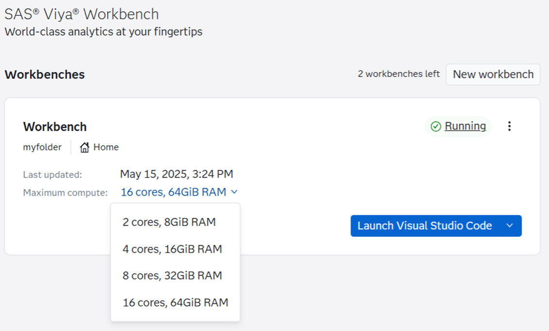
The kitchen
The researchers used a 16-core, 64GB machine with an NVIDIA Tesla C2070 GPU. What I need is the ability to scale with minimal interruption, and SAS Viya Workbench does exactly that. The nice thing about SAS Viya Workbench is that I can choose multiple environment sizes. I can start small and scale up as needed, and it launches almost immediately after I make the change. For this case, we’ll go with a similar environment that the researchers had, especially since we’re working with a nearly 8GB csv file.

Analyzing our ingredients
Before embarking on any modeling mission, we need to see what we’re dealing with:
- Are there any missing values?
- How balanced is the data?
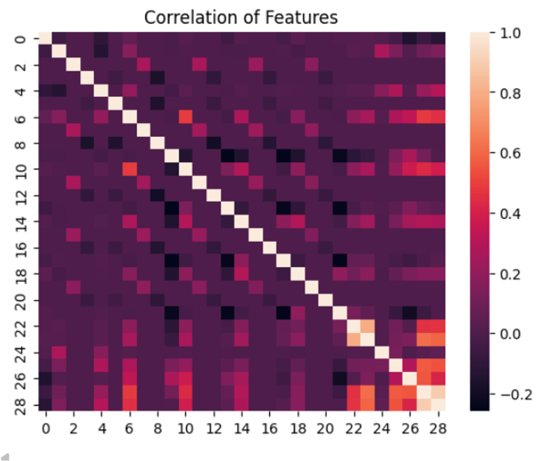
- Is multicollinearity going to be an issue?
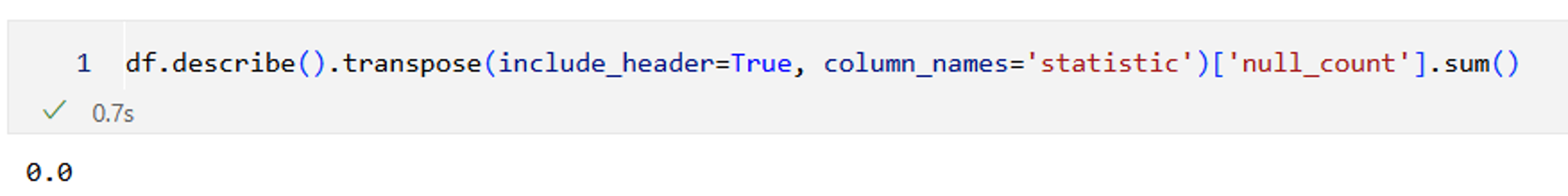
Using a standard data summary, such as described in polars or pandas, we can see there are no missing values of any variables. Perfect.

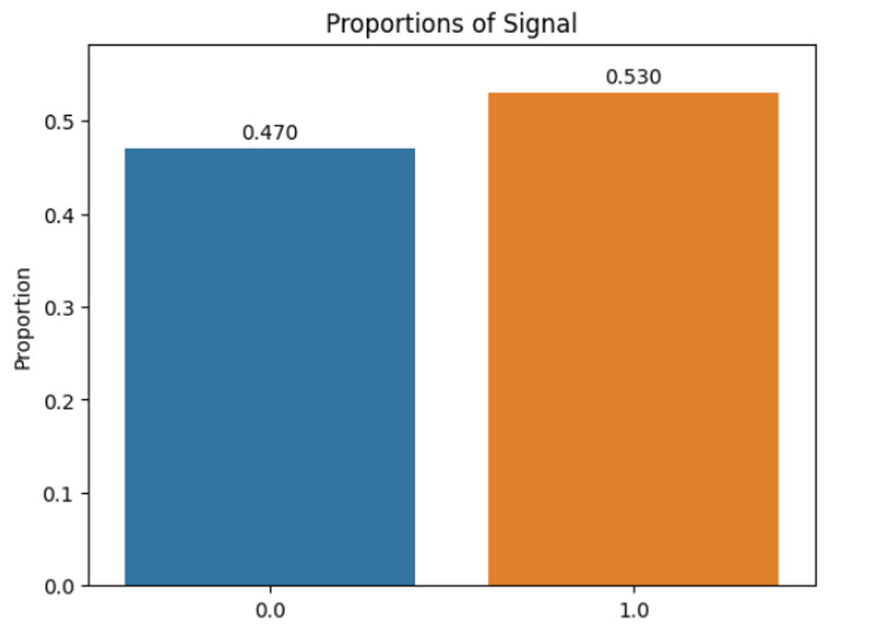
It’s also nearly perfectly balanced with a 47/53 split of background (0)/signal (1).

And almost all variables have low correlation with each other.

The paper already describes the distribution of many of these variables, and in the interest of saving space, I’ll let you take a look at the full Jupyter notebook which graphs out many of these variables. All of them are fairly right-skewed which might mean we want to do some sort of transformation or scaling for our models, but it depends on which model we ultimately choose. But with all of these models out there, which one should we choose?
Bakeoff: what’s the best vanilla cake?
This data is fairly large, and if there’s one thing SAS truly excels at, it’s dealing with big datasets. This is especially true with multi-pass algorithms like gradient boosting or random forest. I did some initial tests with scikit-learn models, and the performance didn’t hold up; some models wouldn’t even finish. So, we’ll be turning to SAS models, which are also compatible with scikit-learn’s utilities to boot.
from sasviya.ml.linear_model import LogisticRegression from sasviya.ml.svm import SVC from sasviya.ml.tree import DecisionTreeClassifier, ForestClassifier, GradientBoostingClassifier |
We’ll do a model bakeoff by running five SAS classification models through the gamut to see which comes out best. Here’s the setup:
- Create a set of pipelines that run default Logistic Regression, Support Vector Machine (SVM), Decision Tree, Random Forest, and Gradient Boosting
- Transform with a Standard Scaler depending upon the model
- Perform 5-fold cross-validation on all 11M observations
- Compare the average accuracy and standard deviation
This is like testing out variations of vanilla cakes before we turn it into something magnificent. The tastiest one wins. Here are the results:
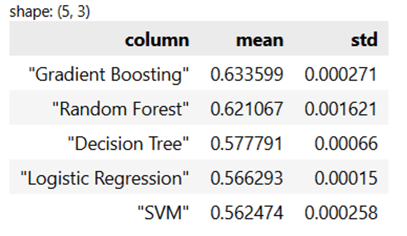


Gradient boosting is the clear winner here, followed closely by random forest. This isn’t too surprising, as tree-based models tend to really shine. Even more impressive is that our standard deviation for accuracy is negligible, meaning there’s strong consistency across all our models.
We’re going to decide on gradient boosting. We don’t care too much about the interpretability of our model. We just want the best-performing, most generalizable model possible. You already know where this is going. Let’s do some hyperparameter autotuning.
Fine-tuning the flavor
We’re going to try tuning the hyperparameters of the gradient boosting model to see if we can get more performance. Not only that, we’re going to do it intelligently: we don’t want to randomly choose values and hope for the best. We want to try values that work and move in a direction that makes sense. This is where Optuna comes in.
Think of Optuna like a smart food critic who looks at every attempt and says “Hmm, that last cake was too dense. Maybe try lowering the oven temperature a bit next time.” It learns from each cake you bake, gradually steering you towards the perfect cake instead of blindly trying every temperature and time combination.
From a technical perspective, Optuna is an open source model-agnostic intelligent hyperparameter autotuning framework that uses Bayesian optimization to choose hyperparameters that work well. It builds a probabilistic model of which hyperparameters might work and tests the most promising ones next. This makes it faster, smarter, and more effective. In a world where time and compute are money, this is more important than ever.
Here’s our plan:
- Split the data into 70% train, 15% validation, and 15% test
- Autotune gradient boosting against the validation set for both low-level and high-level models
- Verify the results with the untouched test dataset
Because we have so much data and because we saw our models performed consistently in k-fold cross-validation, we’re going to tune our hyperparameters against a validation dataset, then confirm it with a test dataset. This is a great way to reduce computing time. Because we have a test dataset, we can make sure that our model is generalizable and not just tuned to the validation dataset.
Optuna, our own personal Gordon Ramsay
To do this, we’ll create a performance objective for Optuna to maximize or minimize, and tell it to run a study on that objective. In other words, we tell Optuna a range of hyperparameters to try, how many times to try a combination, and see what we end up with. It’s kind of like if we had Gordon Ramsay critiquing our cakes and suggesting different ways to improve them based on how it came out last time, just without all the shouting and deeply personal insults.
We’re going to optimize the ROC Area Under the Curve (AUC), which is the same metric that is used in the paper (note that this is different from accuracy that we used above for our initial model selection). If you’re unfamiliar with this metric, check out this comprehensive tutorial from Jeff Thompson about ROC charts in SAS and how to interpret them. All you need to know right now is that a number ranging from 0 to 1. 0.5 means the model is as good as a coin flip, 1 means it predicts perfectly, and anything below 0.5 means it’s worse than random guessing. The closer to 1 you are, the better the model is at distinguishing between signals and background particles. According to the research paper, “small increases in AUC can represent significant enhancement in discovery significance”, so we’ll take any improvements we can get.
def low_level_objective(trial): n_bins = trial.suggest_int('n_bins', 10, 100, step=5) n_estimators = trial.suggest_int('n_estimators', 50, 300, step=10) max_depth = trial.suggest_int('max_depth', 5, 17) min_samples_leaf = trial.suggest_int('min_samples_leaf', 100, 1000, step=50) learning_rate = trial.suggest_float('learning_rate', 0.01, 0.1, step=0.01) model = GradientBoostingClassifier( n_bins = n_bins, n_estimators = n_estimators, max_depth = max_depth, min_samples_leaf = min_samples_leaf, learning_rate = learning_rate, random_state = 42 ) model.fit(X_train_low, y_train) preds = model.predict_proba(X_val_low).iloc(:,1) auc = roc_auc_score(y_val, preds) return auc |
low_level_study = optuna.create_study( direction = 'maximize', study_name = 'Low-level variables: Gradient Boosting Autotuning', ) low_level_study.optimize(low_level_objective, n_trials=30) |
Now all we do is sit back, relax, and let Optuna do all the work.
The final taste test
Two SAS gradient boosting models were tuned: a model with low-level variables and a model with high-level variables. Each model went through 30 trials, meaning we ran 60 variations of gradient boosting models. The SAS models handled all these combinations without any concerns, even as complexity grew drastically. The fact that they handled these dozens of training iterations with ease shows just how well-optimized the platform is for use cases requiring serious compute power.
Optuna comes with some cool graphics. Let’s take a look at the tuning history to see how it learned across trials.

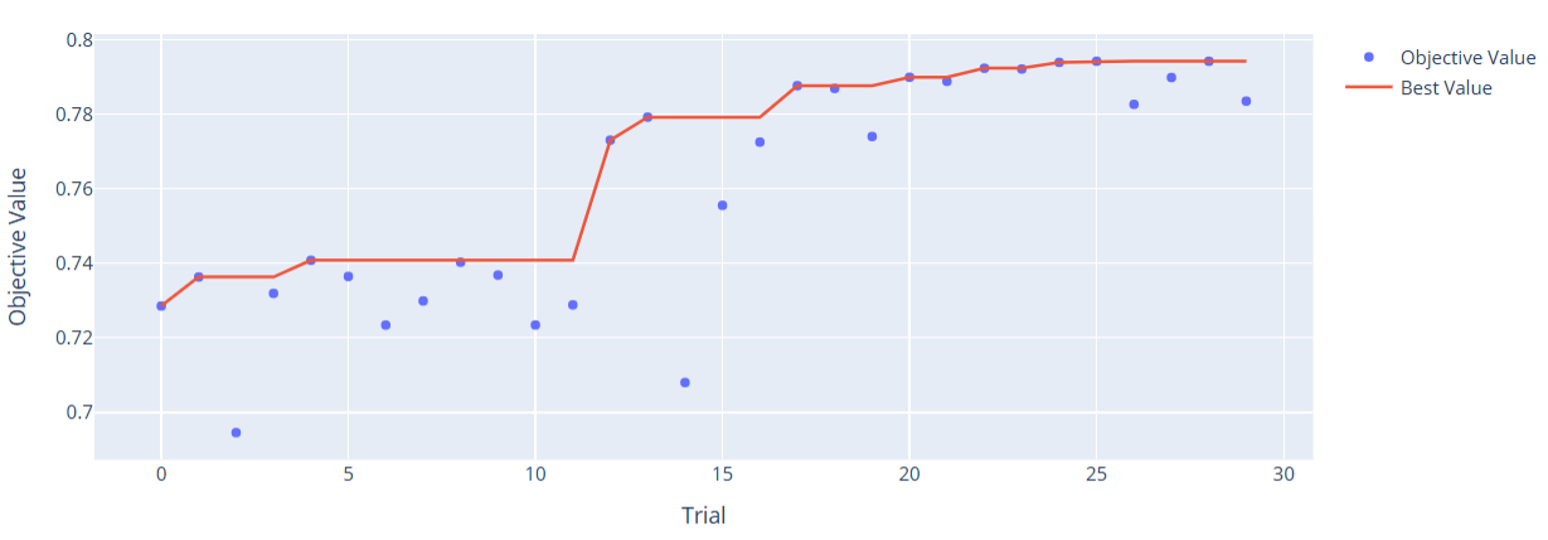

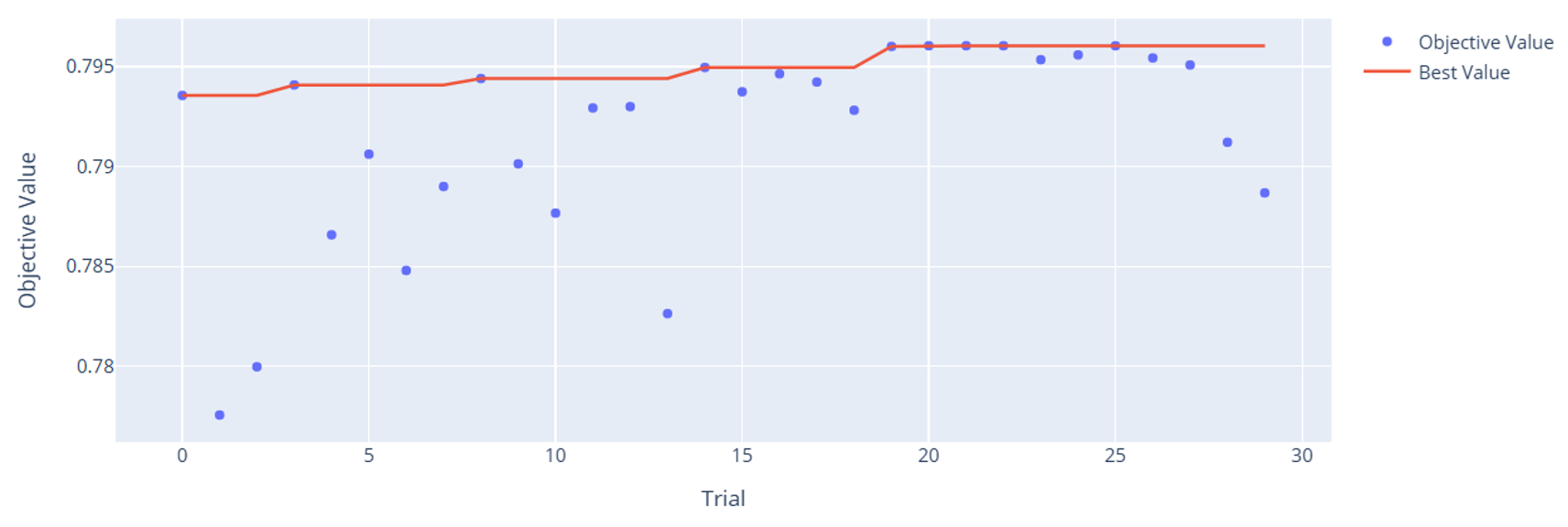
You can very clearly see how Optuna tended to make both models better over time. This is the power of Bayesian hyperparameter autotuning: we don’t need to go through every possible combination. We give it some guard rails, and it will continue trying values that tend to work well. One interesting thing to note is how the high-level variables do such a good job predicting on their own. Remember, these are only 7 variables compared to the 21 raw inputs. It’s a true testament to the deep expertise of particle physicists who can mathematically derive useful variables that improve predictive power over the raw variables alone. This is an important example of how feature engineering using domain knowledge can be massively helpful for improving model performance.
Let’s compare all our models together with both our Validation and Test datasets to see how we did.
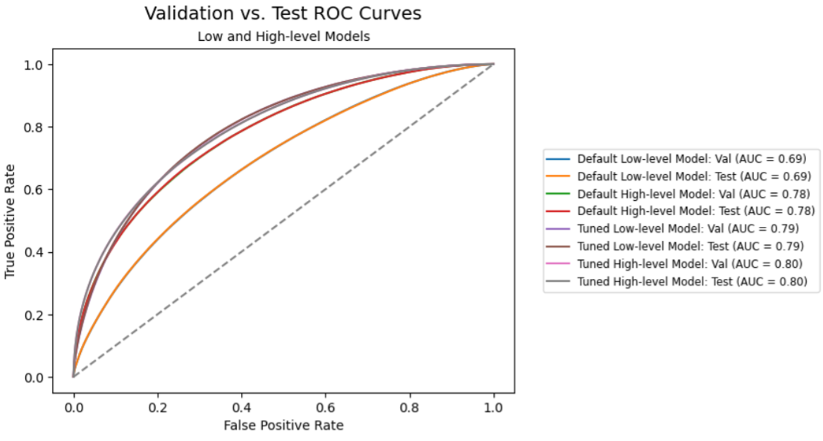

Thanks to hyperparameter autotuning, our champion model’s AUC improved by 15.2% over the gradient boosting model, 8.9% over the boosted decision tree model, and 8.5% over the shallow neural network model. In addition, the results are almost identically consistent between the validation and test datasets. That’s excellent for generalization.
Here’s a breakdown of the tuned gradient boosting model compared to those in the paper:
| Model | AUC: Low-level | Δ vs SAS (%) | AUC: High-level | Δ vs SAS (%) |
| SAS: Tuned Gradient Boosting | 0.795 | 0.796 | ||
| Paper: Boosted Decision Tree | 0.73 | -8.2% | 0.78 | -2.0% |
| Paper: Shallow Neural Network | 0.733 | -7.8% | 0.777 | -2.4% |
| Paper: Deep Neural Network | 0.880 | +10.7% | 0.885 | +11.2% |
The tuned gradient boosting model can’t match the performance of a well-designed, highly-tuned deep neural network, but we were able to do better than both the boosted decision tree and shallow neural network. In the end, we created a low-level model that was as good or better than the high-level model for both the SAS and models, all without a GPU.
Hyperparameter autotuning is a powerful tool for squeezing out extra accuracy, but it comes with trade-offs: increased model complexity, higher risk of overfitting, and reduced interpretability. Not to mention, you’re going to be using more time and computing power. That’s why validation is critical. The more diverse and representative your data, the better your model will generalize. A model that performs well on the training set but falls apart in the real world may have simply learned to predict noise. It’s kind of like fondant: sure, it makes your cake look pretty, but it tastes downright awful.
In our case, we had a large, clean, balanced, and diverse dataset. Our ultimate goal was to improve accuracy, not interpretability, so with all the right conditions in place, autotuning helped get us the most out of our model. Sometimes you really can have your cake and eat it too.