Discovering delays in nonlinear time series with Procsselectlag in Sas Viya

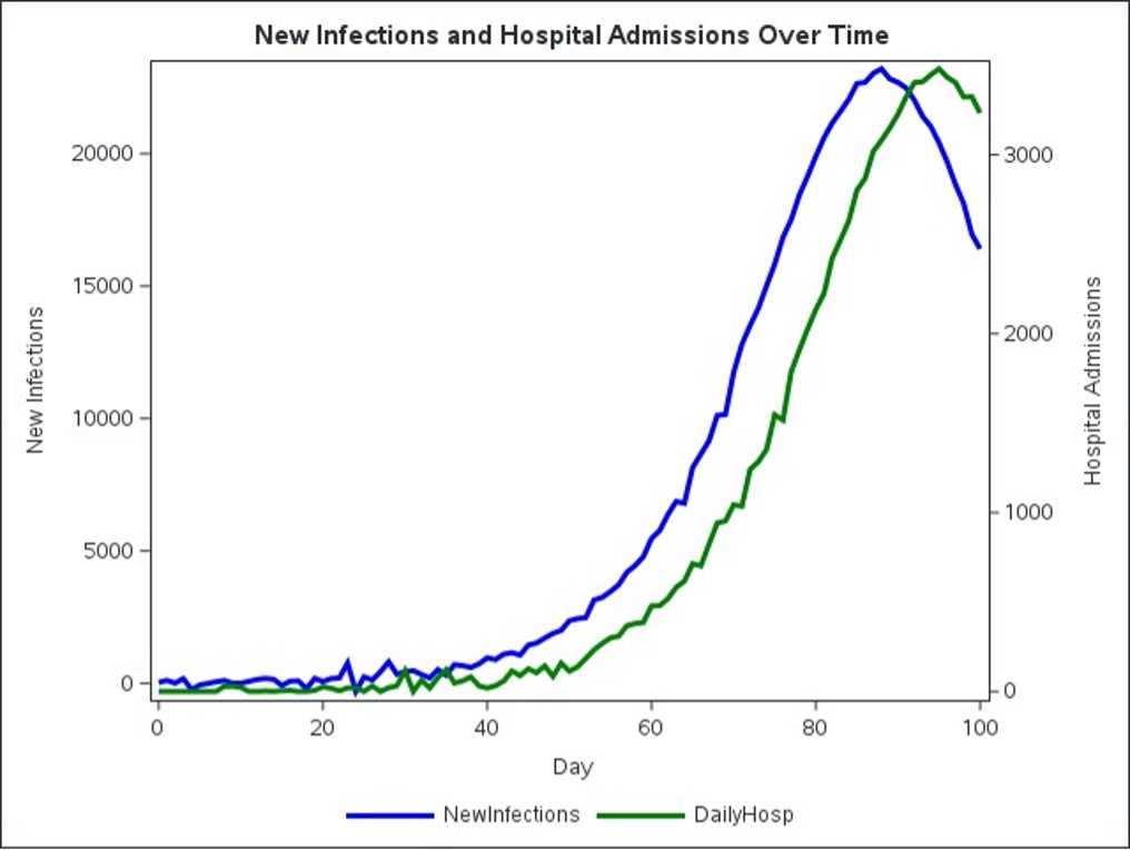
Accurate identification of delays between related time series is essential in forecasting, especially in public health, where delays between events, such as infections and hospital admissions, significantly affect decision -making. Consider a realistic scenario where you need to plan hospital resources based on infection data. In an epidemic, new infections today usually result in hospitalization a few days later, creating a delayed relationship that you need to identify exactly for effective readiness and response. To illustrate this challenge, you will simulate a 100-day epidemic using a seir epidemiological model (sensitive, exposed, infectious, recovered). Seir model captures the progression of infectious disease through distinct stages. In this simulation, you will clearly codify a realistic seven-day delay between new infections and daily admissions to the hospital, including epidemiological parameters such as the level of infection (all over = 0.30), incubation period (on average five days), recovery rate (on average ten days) and hospitalization proportion (15%)-plus random variability to imitate real-world reporting fluctuations.

Figure 1 visually confirms the intended seven-day delay, clearly showing the hospital admissions by constantly following the curve of new infections for about a week.

While visually intuitive, by systematically identifying this delay presents important challenges. Traditional correlation measures – such as Pearson’s correlation – are mainly created for linear relationships and can deceive you in cases that include nonlinear dynamics in the epidemic scenarios. To forcefully detect both linear and nonlinear relationships, you will use the remote correlation, available in Sas Viya through Proc tsselectlag. Distance correlation captures nonlinear complex dependence, providing the most accurate detection of delay structures. Remote correlation mathematically evaluates dependence through the Euclidean distance matrices in the couple. ABOUT UNDER Observations in 2 random variables {(X_deckY_deck) :: deck = 1…, n}, calculate distances in pairs and with their two centers in matrix A_ij AND all over_ijgiving the covariance of empirical distance v_UNDER²(X, y ) and the correlation r_UNDER(X, y ) ::

Remote correlation reliably detects independence and nonlinear associations.

To demonstrate this practically, you will create a CAS session and generate simulated data:

cas mysess; libname mylib cas
sessref=mysess;
 
data mylib.epi(keep=Time NewInfections DailyHosp); call
streaminit(12345);
N=1e6; beta=0.30; sigma=1/5; gamma=1/10; p=0.15; lagH=7; days=100; S=N-200;
E=100; I=100; R=0; array NI(0:1000) _temporary_;
 
do Time = 0 to days;
NewInfections = sigma*E + rand("t",3)*105;
NI(Time)=NewInfections;
 
DailyHosp=0; if Time>=lagH
then do;
DailyHosp=p*NI(Time-lagH)+rand("t",3)*15; if
DailyHosp<0 then DailyHosp=0;
end;
 
dS=-beta*S*I/N; dE=beta*S*I/N - sigma*E; dI=sigma*E -
gamma*I; dR=gamma*I;
S+dS; E+dE; I+dI; R+dR; output; end;
run;
 
ods output Results=pearTbl; proc tsselectlag data=mylib.epi minlag=1 maxlag=14
correlationtype=pearson; id Time; yvar DailyHosp; xvar NewInfections;
run;

Applying the processselectlag with the Pearson correlation incorrectly identifies the strongest correlation in moisture 2 due to the linear assumptions of the Pearson correlation.

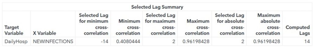
The following call to proc Tsselectlag calculates the bonding of the distance between the delays of new infections and hospitalization in daily hospitals.

ods output Results=distTbl; proc tsselectlag data=mylib.epi minlag=1 maxlag=14
correlationtype=distance; id Time; yvar DailyHosp; xvar NewInfections;
run;

Remote correlation correctly identifies the maximum correlation in neighborhood 7.

Using the remote correlation through ProSelectlag ProC, you will overcome Pearson’s correlation restrictions, accurately capturing nonlinear delay structures essential for reliable prediction. Catching the correct delay structure improves the accuracy of the forecast.

Learn more