Visualize the Gini-Simson Diversity Index

A previous article discusses the Gini-Simson diversity index and how to calculate it in SAS. Suppose you have a sample containing Class R. (Classes are also called groups or categories.) Intuitively, the sample exhibits “high diversity” if class sizes are approximately equal. The sample indicates “low diversity” if class sizes are very different, and especially if there is a large set and small groups R-1. This article visualizes the Gini-Simson diversity index by plotting the index against group sizes. Visualization gives the question in question as “how high (or low) can be the diversity index when my data contains class R?”

Definitions and marking

In this article, n is the number of observations in data and the size of the groups are n₁n₂…, n_with. Gini-Simpson diversity index (GS index, for February) counts as 1-λ where λ is the Simpson Homogeneity Index, defined by

The case when r = 1 is not interesting because λ = 1 (sample is homogeneous), so now assume that R> 1.

What is the diversity index for the most diverse sample?

Let us consider a sample that has N observations, and the size of the R groups is equal. If r is evenly separated, then n_I = N/r for all i. Then the formula for homogeneity index Simpson simplifies

(for equal groups R) From this formula, you can see the following:

If the R groups are equal in size, the Simpson Homogeneity Index is always less than 1/r. For a large sample that has a small number of group (R ≪ n), λ is only slightly less than 1/r, which is an upper limit in the homogeneity index. For example, if there are groups of size R = 3 of equal size, the Simpson homogeneity index is always less than 1/3.

Similarly, if the R groups are equal in size, the Gini-Simpson diversity index, which is 1-ALL, is always greater than 1-1/r = (R-1)/r. For example, if there are groups of size R = 3 of equal size, the GS index is greater than 2/3.

You can use the SAS IML function from the previous article to calculate the Gini-Sympson diversity index for evenly divided data between classes R. For example, the following program uses groups N = 30 and R = 3 where each group contains 10 observations.

proc iml;
/* Input: Vector of counts (n1, n2, ..., nR) 
   Output: a 1x3 vector whose elements are:
         { N = sum of the counts,
           Simpson index of homogeneity,
           Gini-Simpson index of diversity   }
*/
start GiniSimpsonIndex(count);
   Sum = sum(count);
   SimpsonIndex = sum( (count/Sum) # ((count-1)/(Sum-1)) );
   GiniSimpsonIndex = 1 - SimpsonIndex;
   return Sum || SimpsonIndex || GiniSimpsonIndex;
finish;
 
count = {10 10 10};            /* vector of groups sizes */
gs = GiniSimpsonIndex(count);  /* return N, Simpson, Gini-Simpson */
print gs(L="R=3 Even Groups (n_i=10)" c={"N" "Simpson" "Gini-Simpson"});

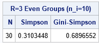
For R = 3 groups of equal size, the Simpson index must be less than 1/3 and the Gini-Sysimson index must be greater than 2/3. Indeed, the calculation indicates that the indices are 0.31 and 0.69, respectively.

The analysis shows that the diversity index depends on the number of groups, R. You can repeat the calculation of indices for n = 30 and for different subgroups:

N = 30;
Rs = {2, 3, 5, 6, 10};           /* number of groups: use numbers that evenly divide N */
labls = {"N" "R" "Group Size (n_i)" "Gini-Simpson Index" "Bound"};
result = j(nrow(Rs), 5, N);  
do i = 1 to nrow(Rs);
   R = Rs(i);                    /* number of groups */
   n_i = N/R;                    /* size of each group */
   LB = (R-1)/R;                 /* a lower bound on the diversity index */
   count = repeat(n_i, 1, R);    /* vector of groups sizes, such as {10 10 10} */
   gs = GiniSimpsonIndex(count); /* return N, Simpson, Gini-Simpson */
   result(i,2:5) = R || n_i || gs(,3) || LB;
end;
print result(L="" c=labls F=BEST7.);

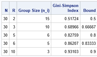
Note that the GS index is always larger than the last column (“connected”). Note also that “connected” depends only on R while the GS index depends on N and R.

Distribution of diversity index for r = 2 classes

The formula for the Gini-Simpson diversity index is challenging to interpret when subgroups are not equal. Let’s visualize the GS index for a fixed size of the sample (N) and a fixed number of groups (R) as the size of the subgroups varies. Without loss of generality, let’s count groups according to their relative sizes. Thus, we assume that n₁ ≥ n₂ ≥ … ≥ n_with > 0. In addition, there are only free R-1 parameters because σ n₁ = N.

The simplest case is R = 2. The largest group must have at least N/2 elements and may have in most N-1 elements. The size of the second group is determined by the equation n₂ = N – n₁. Consequently, the following SAS IML statements calculate the Gini-Simson index for all possible sizes of the two groups. You can then plot the index value as a function of the size of the larger subgroup:

/* run the analysis for all possible (n1,n2) sizes where n1 >= n2 > 0 and n1+n2=30 */
N = 30;
n1 = T( N/2 : (N-1) );         /* sizes for first group */
n2 = N - n1;                   /* sizes for second group */
count = n1 || n2;
*print count(L="Group Sizes" c={'n1' 'n2'});
 
r = j(nrow(count), 3, .);
do i = 1 to nrow(count);
   r(i,) = GiniSimpsonIndex( count(i,) );  
end;
 
/* visualize the Gini-Simpson probability */
result = count || r;
create Diversity2Group from result(c={'n1' 'n2' 'N' 'Simpson' 'GiniSimpson'});
   append from result;
close;
QUIT;
 
title "Diversity Index for Sample with 2 Groups and N=30";
proc sgplot data=Diversity2Group noautolegend;
   needle x=n1 y=GiniSimpson;
   scatter x=n1 y=GiniSimpson / datalabel=GiniSimpson datalabelpos=Top markerattrs=(symbol=CircleFilled);
   xaxis integer values=(15 to 30);
   yaxis offsetmin=0 offsetmax=0.1 grid;
   format GiniSimpson 3.2;
   label GiniSimpson="Gini-Simpson Diversity Index" n1="n1 = Size of Group 1";
run;

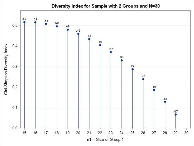
The graph visualizes Gini-Simson diversity statistics for different sizes of two subgroups in a sample of size n = 30. The data is “more diverse” when each subgroup has 15 elements (GS index = 0.52). The index does not differ much for minor deviations from this case. For example, the index is 0.5 when n₁= 18 and n₂= 12. The sample is less varied when the larger subgroup has 29 elements and smaller has an element (index GS = 0.07).

Recall that the GS index is a probability. When the subgroups are equal, there is a probability of 52% that two randomly selected items are in different groups. In the extreme case, there is only a probability of 7% that two randomly selected items are in different groups.

Distribution of diversity index for r = 3 classes

The other simplest case is when there is class R = 3 in the data. For this case, the largest subgroup has a size (n₁) that may vary between observations N/3 and N-2. Values of other subgroups must be positive numbers that are smaller than n₁. The following program generates all possible triplets (n₁n₂n₃) for which n₁ ≥ n₂ ≥ n₃ > 0 and that satisfies n₁ + n₂ + n₃ = N. again, we will choose n = 30 for visualization.

/* run the analysis for R=3 groups and N=30 obs where n1 >= n2 >= n3 > 0 and 
   n1 + n2 + n3 =30 */
N = 30;
n1 = T( N/3 :(N-2) );           /* range of n1 */
n2 = T( 1 : N/2 );              /* size of n2 */
g = expandgrid(n1, n2);         /* possible pairs of (n1,n2) */
c = g || (N - g(,1) - g(,2));   /* possible pairs of (n1,n2,n3) */
isValid = loc(c(,1)>=c(,2) & c(,2)>=c(,3) & c(,3)>0); /* enforce constraints */
count = c(isValid, );
gs = j(nrow(count), 3, .);
do i = 1 to nrow(count);
   gs(i,) = GiniSimpsonIndex( count(i,) );
end;
 
result = count || gs;
create Diversity3Group from result(c={'n1' 'n2' 'n3' 'N' 'Simpson' 'GiniSimpson'});
append from result;
close;
QUIT;

The diversity group3 contains GS statistics for all possible sizes of three subgroups. We can use a heat map to visualize GS statistics as a function of (n₁n₂). To ensure that the color scale includes the entire range (0.1) for the GS index, you can determine a map of the attributes. However, for brevity, I will simply add two false observations to the data: one with the GS index equal to 0 and one with the GS index equal to 1.

data Fake;  /* ensure color model is on (0,1) */
Simpson = 0; GiniSimpson = 0; output;
Simpson = 1; GiniSimpson = 1; output;
run;
 
data Diversity3Group;
set Fake Diversity3Group;
GS = putn(GiniSimpson, 3.2);    /* label for the cells */
run;
 
%let BrBgRamp = CX8C510A CXD8B365 CXF6E8C3 CXF5F5F5 CXC7EAE5 CX5AB4AC CX01665E ;
title "Diversity Index for Sample with 3 Groups and N=30";
title2 "n1 + n2 + n3 = 30"; 
proc sgplot data=Diversity3Group noautolegend;
   heatmapparm x=n1 y=n2 colorresponse=GiniSimpson / name="heat" outline colormodel=(&BrBgRamp);
   gradlegend "heat";
   scatter x=n1 y=n2 / datalabel=GS datalabelpos=center  markerattrs=(size=0);
   xaxis grid integer values=(9 to 29);
   yaxis grid integer values=(0 to 15);
   label GiniSimpson = "Gini-Simpson Diversity Index";
run;

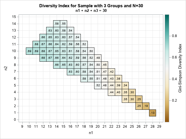
This graph visualizes the GS diversity index range over all possible sizes of the three classes. You can make some observations:

The largest value of the diversity index is 0.69 and occurs when n₁ = n₂ = n₃ = 10.

The diversity index is flat close to the maximum, as shown by the large number of blue cells. For example, when the group sizes are (16, 7, 7), the diversity index is 0.60, which is relatively large.

The diversity index is the probability that two items selected randomly belong to the same group. Therefore, it is useful to ask when the probability is 0.5. The faint white cells are all close to 0.5. For example, the diversity index is 0.5 when class sizes are (20, 8, 2) or (19, 10, 1).

The diversity index is small when there is a large group and two smaller groups. The smallest value is 0.13, which occurs when class sizes are (28, 1, 1). The index increases rapidly when the sizes deviate from that extreme case.

Briefing

The Gini-Simpson diversity index is a variety of a sample that has class R. is the largest (at least 1- 1/r) when all groups are of similar sizes. It is smaller when there is a large group, and other groups all have an observation. This article shows two GS index visualizations, one with groups R = 2 and one with groups R = 3. When class sizes are approximately equal (sample is different), the GS index is not very sensitive to changes in class sizes. However, when class sizes are very different (sample is homogeneous), the GS index is susceptible to changes in class sizes.

Definitions and marking

What is the diversity index for the most diverse sample?

Distribution of diversity index for r = 2 classes

Distribution of diversity index for r = 3 classes

Briefing

Related Posts